REML Implementations of Kernel-based Multi-trait Multi-environment Genomic Prediction Models
Introduction
Linear mixed models for G $\times$ E $\times$ M data
Suppose we have multi-trait genotype by environment (G $\times$ E) or genotype by environment by management (G $\times$ E $\times$ M) data from a multi-environment trial (MET) breeding program:
\[\mathbf{y} = \begin{bmatrix} y_{111} \\ y_{112} \\ \vdots \\ y_{pqr} \\ \end{bmatrix},\]where $r$ genotypes are nested within $q$ environments, which are themselves nested within $p$ traits or managements. Asuming we have BLUEs from first stage analyses and thus a single phenotypic value for every G $\times$ E $\times$ M combination, we have $p \times q \times r = n$ records. We can model this data using a linear mixed model of the following form:
\[\mathbf{y} = \mathbf{X}\boldsymbol{\beta} + \mathbf{Zu} + \boldsymbol{\epsilon},\]where $\mathbf{X} \in \mathbb{R}^{n \times pq}$ is a design matrix for the fixed effects and $\boldsymbol{\beta}$ is the $pq \times 1$ vector containing the estimates of these fixed effects (means of every E $\times$ M combination). The $n \times 1$ vector $\boldsymbol{\epsilon}$ contains the residuals. The design matrix $\mathbf{Z}$ links records to the BLUPs for all G $\times$ E $\times$ M combinations in $\mathbf{u}$. Note that if we have $n$ records and they are ordered correctly, $\mathbf{Z} = \mathbf{I}_n$. The random vector $\mathbf{u}$ follows a multivariate normal distribution:
\[\mathbf{u} \sim \mathcal{N}\left(\mathbf{0}, \boldsymbol{\Sigma}\right),\]where $\boldsymbol{\Sigma}$ is the covariance matrix of $\mathbf{u}$. It is the modeling of this covariance matrix that we are primarily interested in. For G $\times$ E $\times$ M data we typically assume that $\boldsymbol{\Sigma}$ is composed of kronecker products of three smaller covariance matrices, one for each of the three factors genotype, environment, and management:
\[\boldsymbol{\Sigma} = \boldsymbol{\Sigma}_{M} \otimes \boldsymbol{\Sigma}_{E} \otimes \boldsymbol{\Sigma}_{G}.\]The matrix $\boldsymbol{\Sigma}_{G}$ is easy to model; we can use the genomic kinship matrix $\mathbf{K}$ or pedigree-based relationship matrix $\mathbf{A}$. We will assume that $\boldsymbol{\Sigma}_{G} = \mathbf{K}$ from here on. The matrices $\boldsymbol{\Sigma}_{M}$ and $\boldsymbol{\Sigma}_{E}$ are trickier. There are usually only a relatively small number of managements or traits, e.g., low vs medium vs high nitrogen, irrigated vs rainfed, or plant height and yield. We can thus use an unstructured model for $\boldsymbol{\Sigma}_{M}$ as we only need to estimate a few correlations. The covariance matrix of environments $\boldsymbol{\Sigma}_{E}$ is the hardest to model. As we typically have a relatively large number of environments, an unstructured model quickly becomes infeasible. In that case, a factor analytic (FA) structure is a popular choice. FA structures can still be problematic, however. Practically speaking, the model with the double kronecker product between an unstructured matrix for M, an FA matrix for E, and the kinship for G is very hard to fit. A solution that is often used is combining M and E into a new factor that is modeled using a single covariance matrix:
\[\mathbf{u} \sim \mathcal{N}\left(\mathbf{0}, \boldsymbol{\Sigma}_{ME} \otimes \mathbf{K}\right),\]where an FA structure is used for $\boldsymbol{\Sigma}_{ME}$. While this works better, estimation of $\boldsymbol{\Sigma}_{ME}$ can still be challenging if there is a large number of environments or if not all genotypes are present in all environments due to an MET design called sparse testing (see this paper for some information on sparse testing).
Using kernels to model G $\times$ E $\times$ M data
A possible solution to the challenges outlined in the previous section is to use environmental covariables. These can be used in several ways, but here we use them to construct kernels that model additive genetic correlations between environments without having to estimate a large number of parameters. The kernels can be thought of as kinship matrices for environments that are calculated using environmental covariables, instead of using genomic SNP markers for a genomic kinship matrix. There are several options when using these kernels. They can be linear or non-linear functions of environmental covariables. We can combine them with additive genetic variances for each management (thus assuming the same variance for all environments within that management), or model a unique variance for every E $\times$ M combination. The same options are available when modeling multi-trait G $\times$ E data. Another nice thing about these kernels is that we can do everything in standard software, ASReml-R in this case.
The remainder of this page contains several R functions that construct covariance matrices and partial derivatives using linear and non-linear kernels built with environmental covariables.
There are functions for modeling a single variance for all environments within a level of management or trait, as well as functions for modeling variances for all combinations.
The functions are meant to be used with the own() function in ASReml-R for modeling (G $\times$ E $\times$ M) or multi-trait G $\times$ E data.
While these functions are practically plug & play, there are two important things to keep in mind:
-
The linear kernel supplied by the user must be a numeric matrix object called
Cthat exists in the global environment. For the non-linear kernels, the user-supplied distance matrices must be calledD. This can be changed by modifying the functions, i.e., replacingCandDwith whatever other name one wants to use. Just make sure that R will find the correct object in the global environment. Do not defineCorDwithin the variance function. This works because when R cannot find referenced objects within the local environment of the function, it simply looks in the enclosing environment (the environment where the function was defined), whereCorDexists (see this page for more information). -
The row- and column order of
CandD, must match the order of the levels of the environment factor in the dataframe that is passed to ASReml-R:
C <- C[levels(data$Environment), levels(data$Environment)]
Another option is to use the cornfruit package that provides wrappers around the functions, taking care of point 1. See the end of this page for more information.
Linear kernels
The linear kernels are computed similarly to how a genomic relationship matrix is obtained:
\[\mathbf{C} = \dfrac{\mathbf{W}^\top\mathbf{W}}{w-1},\]where $\mathbf{W}$ is a column-wise centered and scaled $w \times q$ matrix containing $w$ environmental covariables for $q$ environments. Simply put, a linear kernel is a correlation matrix of environments, based on environmental covariables. The kernel $\mathbf{C}$ can then be combined with a single variance for each management or trait, or unique variance for all environments within a given management or trait.
Single variance linear kernel (svlk)
The single variance linear kernel assumes the following distribution for $\mathbf{u}$:
\[\mathbf{u} \sim \mathcal{N}\left(\mathbf{0}, \boldsymbol{\Sigma}_{M} \otimes \mathbf{C} \otimes \mathbf{K}\right),\]where $\mathbf{C}$ is the linear kernel described earlier. The covariance matrix $\boldsymbol{\Sigma}_{M}$ is unstructured and estimated like how ASReml-R would estimate a covariance matrix using corgh(). As a simple illustration, consider the case of two managements and two environments:
The parameters to be estimated in the above example are:
\[\boldsymbol{\kappa} = \begin{bmatrix} v_1, v_2, \rho_{12} \end{bmatrix}.\]To estimate these parameters we need the partial derivatives of $\boldsymbol{\Sigma}_M \otimes \mathbf{C}$ with respect to each parameter:
\[\begin{split} \dfrac{\partial \left(\boldsymbol{\Sigma}_M \otimes \mathbf{C}\right)}{\partial v_1} &= \begin{bmatrix} \mathbf{C}_{11} & \mathbf{C}_{12} & \dfrac{0.5\,\sqrt{v_2}\,\rho_{12}\,\mathbf{C}_{11}}{\sqrt{v_1}} & \dfrac{0.5\,\sqrt{v_2}\,\rho_{12}\,\mathbf{C}_{12}}{\sqrt{v_1}} \\[10pt] \mathbf{C}_{21} & \mathbf{C}_{22} & \dfrac{0.5\,\sqrt{v_2}\,\rho_{12}\,\mathbf{C}_{21}}{\sqrt{v_1}} & \dfrac{0.5\,\sqrt{v_2}\,\rho_{12}\,\mathbf{C}_{22}}{\sqrt{v_1}} \\[10pt] \dfrac{0.5\,\sqrt{v_2}\,\rho_{12}\,\mathbf{C}_{11}}{\sqrt{v_1}} & \dfrac{0.5\,\sqrt{v_2}\,\rho_{12}\,\mathbf{C}_{12}}{\sqrt{v_1}} & 0 & 0 \\[10pt] \dfrac{0.5\,\sqrt{v_2}\,\rho_{12}\,\mathbf{C}_{21}}{\sqrt{v_1}} & \dfrac{0.5\,\sqrt{v_2}\,\rho_{12}\,\mathbf{C}_{22}}{\sqrt{v_1}} & 0 & 0 \end{bmatrix} \\ \\ \dfrac{\partial \left(\boldsymbol{\Sigma}_M \otimes \mathbf{C}\right)}{\partial v_2} &= \begin{bmatrix} 0 & 0 & \dfrac{0.5\,\sqrt{v_1}\,\rho_{12}\,\mathbf{C}_{11}}{\sqrt{v_2}} & \dfrac{0.5\,\sqrt{v_1}\,\rho_{12}\,\mathbf{C}_{12}}{\sqrt{v_2}} \\[10pt] 0 & 0 & \dfrac{0.5\,\sqrt{v_1}\,\rho_{12}\,\mathbf{C}_{21}}{\sqrt{v_2}} & \dfrac{0.5\,\sqrt{v_1}\,\rho_{12}\,\mathbf{C}_{22}}{\sqrt{v_2}} \\[10pt] \dfrac{0.5\,\sqrt{v_1}\,\rho_{12}\,\mathbf{C}_{11}}{\sqrt{v_2}} & \dfrac{0.5\,\sqrt{v_1}\,\rho_{12}\,\mathbf{C}_{12}}{\sqrt{v_2}} & \mathbf{C}_{11} & \mathbf{C}_{12} \\[10pt] \dfrac{0.5\,\sqrt{v_1}\,\rho_{12}\,\mathbf{C}_{21}}{\sqrt{v_2}} & \dfrac{0.5\,\sqrt{v_1}\,\rho_{12}\,\mathbf{C}_{22}}{\sqrt{v_2}} & \mathbf{C}_{21} & \mathbf{C}_{22} \end{bmatrix} \\ \\ \dfrac{\partial \left(\boldsymbol{\Sigma}_M \otimes \mathbf{C}\right)}{\partial \rho_{12}} &= \begin{bmatrix} 0 & 0 & \sqrt{v_1}\,\sqrt{v_2}\,\mathbf{C}_{11} & \sqrt{v_1}\,\sqrt{v_2}\,\mathbf{C}_{12} \\[5pt] 0 & 0 & \sqrt{v_1}\,\sqrt{v_2}\,\mathbf{C}_{21} & \sqrt{v_1}\,\sqrt{v_2}\,\mathbf{C}_{22} \\[5pt] \sqrt{v_1}\,\sqrt{v_2}\,\mathbf{C}_{11} & \sqrt{v_1}\,\sqrt{v_2}\,\mathbf{C}_{12} & 0 & 0 \\[5pt] \sqrt{v_1}\,\sqrt{v_2}\,\mathbf{C}_{21} & \sqrt{v_1}\,\sqrt{v_2}\,\mathbf{C}_{22} & 0 & 0 \end{bmatrix}. \end{split}\]Note that this readily generalizes to any number of managements or environments. The R function below automatically computes the covariance matrix $\boldsymbol{\Sigma}_M \otimes \mathbf{C}$ and its partial derivatives:
# kappa[1] = variance for all environments within management 1
# kappa[2] = variance for all environments within management 2
# ...
# kappa[p] = variance for all environments within management p
# kappa[p + 1] = correlation between management 1 and management 2
# ...
# kappa[p + ((p^2 - p) / 2)] = correlation between management p - 1 and management p

vf <- function(order, kappa) {
  # The correlation matrix of the managements:
  q <- nrow(C)
  p <- order / q
  Ct <- matrix(1, p, p)
  Ct[lower.tri(Ct)] <- kappa[(p + 1):(p + ((p^2 - p) / 2))]
  Ct <- Ct + t(Ct) - diag(p)

  # The full covariance matrix:
  S <- outer(sqrt(kappa[1:p]), sqrt(kappa[1:p]))
  V <- kronecker(S * Ct, C)

  # Derivatives wrt kappa[1:p] (variances):
  varderivs <- vector("list", p)
  for (dk in 1:p) {
    I <- matrix(0, p, p)
    I[dk,] <- I[, dk] <- 1
    I <- kronecker(I, matrix(1, q, q))
    tmp <- sqrt(kappa[1:p])
    tmp[dk] <- 1 / tmp[dk]
    tmp <- outer(tmp, tmp)
    tmp[dk, dk] <- 1
    deriv <- 0.5 * I * kronecker(tmp * Ct, C)
    deriv[((dk - 1) * q + 1):(dk * q), ((dk - 1) * q + 1):(dk * q)] <-
      deriv[((dk - 1) * q + 1):(dk * q), ((dk - 1) * q + 1):(dk * q)] * 2
    varderivs[[dk]] <- deriv
  }

  # Derivatives wrt kappa[(p + 1):(p + ((p^2 - p) / 2))] (correlations):
  corderivs <- vector("list", (p^2 - p) / 2)
  for (dk in 1:((p^2 - p) / 2)) {
    # Indicator matrix of where kappa[dk] is present:
    I <- matrix(0, p, p)
    I[lower.tri(I)][dk] <- 1
    I <- I + t(I)
    corderivs[[dk]] <- kronecker(S * I, C)
  }

  return(c(list(V), varderivs, corderivs))
}
and can be used with ASReml-R using the following code:
p <- length(levels(data$Management)) # Number of managements

init <- c(rep(0.1, p), rep(0.1, (p^2 - p) / 2)) # Initial values for the p variances and (p^2 - p) / 2 correlations
type <- c(rep("V", p), rep("R", (p^2 - p) / 2)) # Parameter types
cons <- c(rep("P", p), rep("U", (p^2 - p) / 2)) # Constraints

fit <- asreml(fixed = Y ~ -1 + ManagementEnvironment,
              random = ~ own(ManagementEnvironment, "vf", init, type, cons):vm(Genotype, K),
              residual = ~ units,
              data = data)
assuming that data is a dataframe with columns containing the factor levels for Management, Environment, Genotype, and an extra column with the levels for a factor combining Management and Environment (ManagementEnvironment).
Variance components can be retrieved as usual (summary(fit)$varcomp).
There will not be any descriptive rownames for the variance components, so refer to the comments above the vf() function definition above to see which variance components correspond to which parameters.
For example, the first variance component will correspond to the variance for all environments within the first level of management.
Multiple variance linear kernel (mvlk)
The multiple variance linear kernel assumes the following distribution for $\mathbf{u}$:
\[\mathbf{u} \sim \mathcal{N}\left(\mathbf{0}, \mathbf{s}\mathbf{s}^\top \circ \left(\mathbf{C}_{M} \otimes \mathbf{C}\right) \otimes \mathbf{K}\right),\]where $\mathbf{C}$ is the linear kernel described earlier. The correlation matrix $\mathbf{C}_{M}$ is unstructured and estimated like how ASReml-R would estimate a correlation matrix using corg().
The vector $\mathbf{s}$ contains the standard deviations for each E $\times$ M combination.
As a simple illustration, consider again the case of two managements and two environments:
The parameters to be estimated in the above example are:
\[\boldsymbol{\kappa} = \begin{bmatrix} v_1, v_2, v_3, v_4, \rho_{12} \end{bmatrix}.\]To estimate these parameters we need the partial derivatives of $\mathbf{s}\mathbf{s}^\top \circ \left(\mathbf{C}_M \otimes \mathbf{C}\right)$ with respect to each parameter:
\[\begin{split} \dfrac{\partial \left(\mathbf{s}\mathbf{s}^\top \circ \left(\mathbf{C}_M \otimes \mathbf{C}\right)\right)}{\partial v_1} &= \begin{bmatrix} \mathbf{C}_{11} & \dfrac{0.5\,\sqrt{v_2}\,\mathbf{C}_{12}}{\sqrt{v_1}} & \dfrac{0.5\,\sqrt{v_3}\,\rho_{12}\,\mathbf{C}_{11}}{\sqrt{v_1}} & \dfrac{0.5\,\sqrt{v_4}\,\rho_{12}\,\mathbf{C}_{12}}{\sqrt{v_1}} \\[10pt] \dfrac{0.5\,\sqrt{v_2}\,\mathbf{C}_{21}}{\sqrt{v_1}} & 0 & 0 & 0 \\[10pt] \dfrac{0.5\,\sqrt{v_3}\,\rho_{12}\,\mathbf{C}_{11}}{\sqrt{v_1}} & 0 & 0 & 0 \\[10pt] \dfrac{0.5\,\sqrt{v_4}\,\rho_{12}\,\mathbf{C}_{21}}{\sqrt{v_1}} & 0 & 0 & 0 \end{bmatrix} \\ \\ \dfrac{\partial \left(\mathbf{s}\mathbf{s}^\top \circ \left(\mathbf{C}_M \otimes \mathbf{C}\right)\right)}{\partial v_2} &= \begin{bmatrix} 0 & \dfrac{0.5\,\sqrt{v_1}\,\mathbf{C}_{12}}{\sqrt{v_2}} & 0 & 0 \\[10pt] \dfrac{0.5\,\sqrt{v_1}\,\mathbf{C}_{21}}{\sqrt{v_2}} & \mathbf{C}_{22} & \dfrac{0.5\,\sqrt{v_3}\,\rho_{12}\,\mathbf{C}_{21}}{\sqrt{v_2}} & \dfrac{0.5\,\sqrt{v_4}\,\rho_{12}\,\mathbf{C}_{22}}{\sqrt{v_2}} \\[10pt] 0 & \dfrac{0.5\,\sqrt{v_3}\,\rho_{12}\,\mathbf{C}_{12}}{\sqrt{v_2}} & 0 & 0 \\[10pt] 0 & \dfrac{0.5\,\sqrt{v_4}\,\rho_{12}\,\mathbf{C}_{22}}{\sqrt{v_2}} & 0 & 0 \end{bmatrix} \\ \\ \dfrac{\partial \left(\mathbf{s}\mathbf{s}^\top \circ \left(\mathbf{C}_M \otimes \mathbf{C}\right)\right)}{\partial v_3} &= \begin{bmatrix} 0 & 0 & \dfrac{0.5\,\sqrt{v_1}\,\rho_{12}\,\mathbf{C}_{11}}{\sqrt{v_3}} & 0 \\[10pt] 0 & 0 & \dfrac{0.5\,\sqrt{v_2}\,\rho_{12}\,\mathbf{C}_{21}}{\sqrt{v_3}} & 0 \\[10pt] \dfrac{0.5\,\sqrt{v_1}\,\rho_{12}\,\mathbf{C}_{11}}{\sqrt{v_3}} & \dfrac{0.5\,\sqrt{v_2}\,\rho_{12}\,\mathbf{C}_{12}}{\sqrt{v_3}} & \mathbf{C}_{11} & \dfrac{0.5\,\sqrt{v_4}\,\mathbf{C}_{12}}{\sqrt{v_3}} \\[10pt] 0 & 0 & \dfrac{0.5\,\sqrt{v_4}\,\mathbf{C}_{21}}{\sqrt{v_3}} & 0 \end{bmatrix} \\ \\ \dfrac{\partial \left(\mathbf{s}\mathbf{s}^\top \circ \left(\mathbf{C}_M \otimes \mathbf{C}\right)\right)}{\partial v_4} &= \begin{bmatrix} 0 & 0 & 0 & \dfrac{0.5\,\sqrt{v_1}\,\rho_{12}\,\mathbf{C}_{12}}{\sqrt{v_4}} \\[10pt] 0 & 0 & 0 & \dfrac{0.5\,\sqrt{v_2}\,\rho_{12}\,\mathbf{C}_{22}}{\sqrt{v_4}} \\[10pt] 0 & 0 & 0 & \dfrac{0.5\,\sqrt{v_3}\,\mathbf{C}_{12}}{\sqrt{v_4}} \\[10pt] \dfrac{0.5\,\sqrt{v_1}\,\rho_{12}\,\mathbf{C}_{21}}{\sqrt{v_4}} & \dfrac{0.5\,\sqrt{v_2}\,\rho_{12}\,\mathbf{C}_{22}}{\sqrt{v_4}} & \dfrac{0.5\,\sqrt{v_3}\,\mathbf{C}_{21}}{\sqrt{v_4}} & \mathbf{C}_{22} \end{bmatrix} \\ \\ \dfrac{\partial \left(\mathbf{s}\mathbf{s}^\top \circ \left(\mathbf{C}_M \otimes \mathbf{C}\right)\right)}{\partial \rho_{12}} &= \begin{bmatrix} 0 & 0 & \sqrt{v_1}\,\sqrt{v_3}\,\mathbf{C}_{11} & \sqrt{v_1}\,\sqrt{v_4}\,\mathbf{C}_{12} \\[10pt] 0 & 0 & \sqrt{v_2}\,\sqrt{v_3}\,\mathbf{C}_{21} & \sqrt{v_2}\,\sqrt{v_4}\,\mathbf{C}_{22} \\[10pt] \sqrt{v_1}\,\sqrt{v_3}\,\mathbf{C}_{11} & \sqrt{v_2}\,\sqrt{v_3}\,\mathbf{C}_{12} & 0 & 0 \\[10pt] \sqrt{v_1}\,\sqrt{v_4}\,\mathbf{C}_{21} & \sqrt{v_2}\,\sqrt{v_4}\,\mathbf{C}_{22} & 0 & 0 \end{bmatrix}. \end{split}\]The R function below automatically computes the covariance matrix $\mathbf{s}\mathbf{s}^\top \circ \left(\mathbf{C}_M \otimes \mathbf{C}\right)$ and its partial derivatives:
# kappa[1] = variance for management 1, environment 1
# kappa[2] = variance for management 1, environment 2
# ...
# kappa[p * q] = variance for management p, environment q
# kappa[p * q + 1] = correlation between management 1 and management 2
# ...
# kappa[p * q + ((p^2 - p) / 2)] = correlation between management p - 1 and management p
# order = p * q

vf <- function(order, kappa) {
  # The correlation matrix of the traits:
  q <- nrow(C)
  p <- order / q
  Ct <- matrix(1, p, p)
  Ct[lower.tri(Ct)] <- kappa[(order + 1):(order + ((p^2 - p) / 2))]
  Ct <- Ct + t(Ct) - diag(p)

  # The full covariance matrix:
  S <- outer(sqrt(kappa[1:order]), sqrt(kappa[1:order]))
  V <- S * kronecker(Ct, C)

  # Derivatives wrt kappa[1:(p * q)] (variances):
  varderivs <- vector("list", order)
  for (dk in 1:order) {
    I <- matrix(0, order, order)
    I[dk,] <- I[, dk] <- 1
    tmp <- sqrt(kappa[1:order])
    tmp[dk] <- 1 / tmp[dk]
    tmp <- outer(tmp, tmp)
    tmp[dk, dk] <- 1
    deriv <- 0.5 * I * tmp * kronecker(Ct, C)
    deriv[dk, dk] <- 1
    varderivs[[dk]] <- deriv
  }

  # Derivatives wrt kappa[(p + 1):(p + ((p^2 - p) / 2))] (correlations):
  corderivs <- vector("list", (p^2 - p) / 2)
  for (dk in 1:((p^2 - p) / 2)) {
    # Indicator matrix of where kappa[dk] is present:
    I <- matrix(0, p, p)
    I[lower.tri(I)][dk] <- 1
    I <- I + t(I)
    corderivs[[dk]] <- S * kronecker(I, C)
  }

  return(c(list(V), varderivs, corderivs))
}
and can be used with ASReml-R using the following code:
p <- length(levels(data$Management)) # Number of managements
q <- length(levels(data$Environment)) # Number of environments

init <- c(rep(0.1, p * q), rep(0.1, (p^2 - p) / 2)) # Initial values for the p * q variances and (p^2 - p) / 2 correlations
type <- c(rep("V", p * q), rep("R", (p^2 - p) / 2)) # Parameter types
cons <- c(rep("P", p * q), rep("U", (p^2 - p) / 2)) # Constraints

fit <- asreml(fixed = Y ~ -1 + ManagementEnvironment,
              random = ~ own(ManagementEnvironment, "vf", init, type, cons):vm(Genotype, K),
              residual = ~ units,
              data = data)
Note that in this case, the first variance component is the variance of the first environment within the first level of management.
Non-linear kernels
Linear kernels completely fix the structure of the G $\times$ E pattern, as well as the absolute values of the correlations between environments. This is not particularly flexible and can result in inaccurate predictions if environmental covariables if the linear kernel does not match the true G $\times$ E structure. Non-linear kernels aim to solve this issue by introducing a single parameter called bandwidth that governs how a squared Euclidian distance matrix of the environments, $\mathbf{D}$, is non-linearly transformed into a correlation matrix:
\[\mathbf{C}_E = e^{-h\,\mathbf{D}},\]where $h$ is the bandwidth and
\[\mathbf{D} = \begin{bmatrix} \mathbf{D}_{11} & \dots & \mathbf{D}_{1q} \\ \vdots & \ddots & \vdots \\ \mathbf{D}_{q1} & \dots & \mathbf{D}_{qq} \end{bmatrix},\]where
\[\mathbf{D}_{ij} = \dfrac{1}{w}\sum_{m=1}^{w} \left(\mathbf{W}_{mi} - \mathbf{W}_{mj}\right)^2.\]The matrix $\mathbf{W} \in \mathbb{R}^{w \times q}$ containing values of $w$ environmental covariables for $q$ environments is row-wise centered and scaled. This type of non-linear kernel is often referred to as a Gaussian kernel.
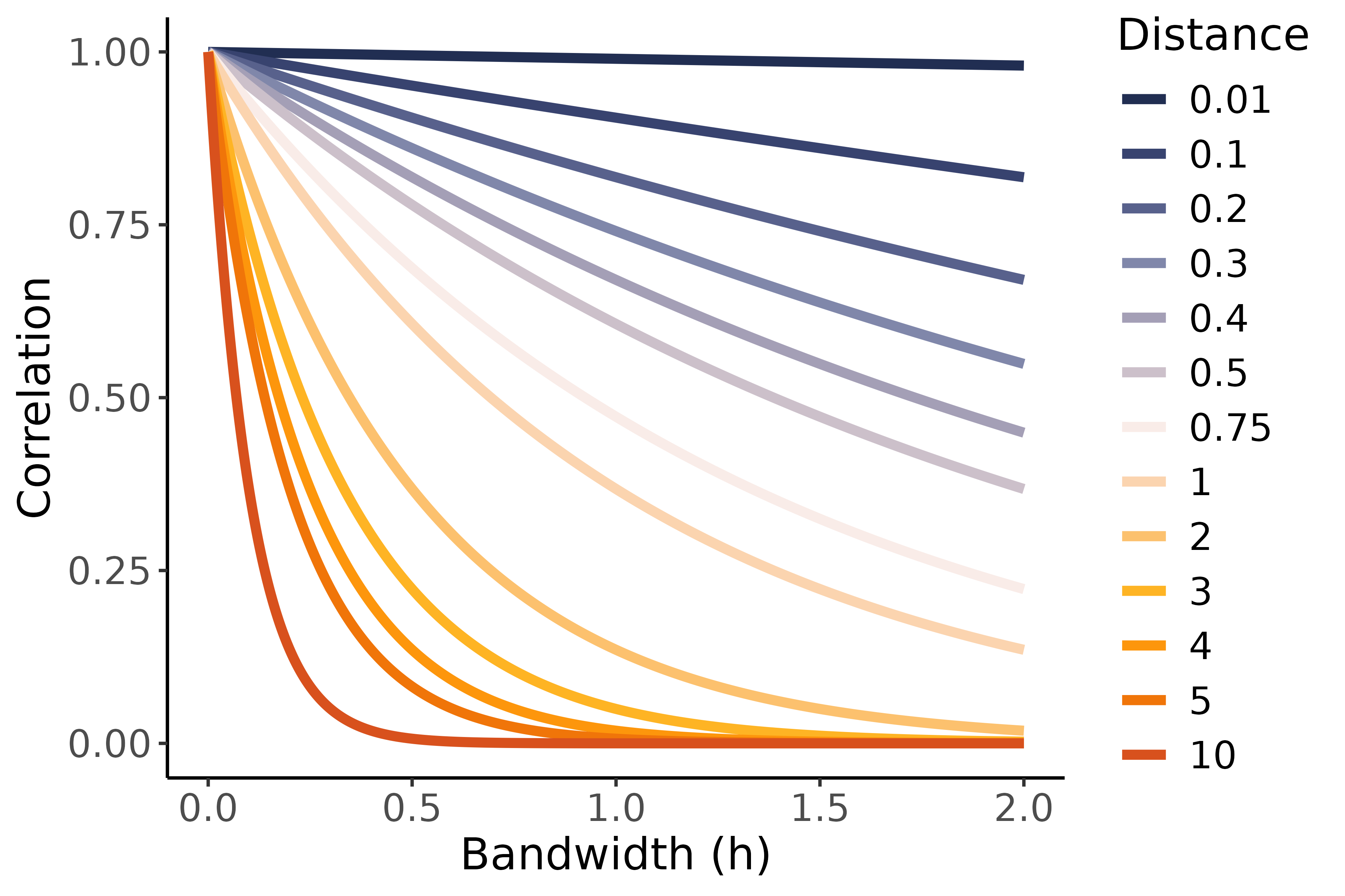
The graph on the right shows the effect of different bandwidth values on the correlations between environments for different squared Euclidian distances. Note that using a non-linear (Gaussian) kernel, only positive correlations between environments can be modeled. Also note that if we treat the bandwidth the same as a variance during estimation, we can end up with either a diagonal or main effects model for the G $\times$ E. If the estimated bandwidth is large, all distances tend to be transformed into correlations close to $0$, leading to a diagonal model where no borrowing of information between environments is happening. Alternatively, if the estimated bandwidth is small, all correlations will tend to be close to $1$ after the non-linear transformation, leading to what is effectively a main effects model that ignores G $\times$ E and allows full borrowing of information between environments. Neither of these extremes are likely to result in good fits, so typically an intermediate bandwidth is estimated such that the correlation matrix obtained after transformation of the distance matrix using that bandwidth fits the data well.
Single variance non-linear kernel (svgk)
The single variance non-linear, or gaussian, kernel assumes the following distribution for $\mathbf{u}$:
\[\mathbf{u} \sim \mathcal{N}\left(\mathbf{0}, \boldsymbol{\Sigma}_{M} \otimes e^{-h\,\mathbf{D}} \otimes \mathbf{K}\right)\]where $\mathbf{D}$ is the squared Euclidian distance matrix of the environments and $h$ is the bandwidth parameter. The covariance matrix $\boldsymbol{\Sigma}_{M}$ is unstructured and estimated like how ASReml-R would estimate a covariance matrix using corgh(). As a simple illustration, consider the case of two managements and two environments:
The parameters to be estimated in the above example are:
\[\boldsymbol{\kappa} = \begin{bmatrix} v_1, v_2, \rho_{12}, h \end{bmatrix}.\]To estimate these parameters we need the partial derivatives of $\boldsymbol{\Sigma}_{M} \otimes e^{-h\,\mathbf{D}}$ with respect to each parameter:
\[\begin{split} \dfrac{\partial \left(\boldsymbol{\Sigma}_{M} \otimes e^{-h\,\mathbf{D}}\right)}{\partial v_1} &= \begin{bmatrix} e^{-h\,\mathbf{D}_{11}} & e^{-h\,\mathbf{D}_{12}} & \dfrac{0.5\,\sqrt{v_2}\,\rho_{12}\,e^{-h\,\mathbf{D}_{11}}}{\sqrt{v_1}} & \dfrac{0.5\,\sqrt{v_2}\,\rho_{12}\,e^{-h\,\mathbf{D}_{12}}}{\sqrt{v_1}} \\[10pt] e^{-h\,\mathbf{D}_{21}} & e^{-h\,\mathbf{D}_{22}} & \dfrac{0.5\,\sqrt{v_2}\,\rho_{12}\,e^{-h\,\mathbf{D}_{21}}}{\sqrt{v_1}} & \dfrac{0.5\,\sqrt{v_2}\,\rho_{12}\,e^{-h\,\mathbf{D}_{22}}}{\sqrt{v_1}} \\[10pt] \dfrac{0.5\,\sqrt{v_2}\,\rho_{12}\,e^{-h\,\mathbf{D}_{11}}}{\sqrt{v_1}} & \dfrac{0.5\,\sqrt{v_2}\,\rho_{12}\,e^{-h\,\mathbf{D}_{12}}}{\sqrt{v_1}} & 0 & 0 \\[10pt] \dfrac{0.5\,\sqrt{v_2}\,\rho_{12}\,e^{-h\,\mathbf{D}_{21}}}{\sqrt{v_1}} & \dfrac{0.5\,\sqrt{v_2}\,\rho_{12}\,e^{-h\,\mathbf{D}_{22}}}{\sqrt{v_1}} & 0 & 0 \end{bmatrix} \\ \\ \dfrac{\partial \left(\boldsymbol{\Sigma}_{M} \otimes e^{-h\,\mathbf{D}}\right)}{\partial v_2} &= \begin{bmatrix} 0 & 0 & \dfrac{0.5\,\sqrt{v_1}\,\rho_{12}\,e^{-h\,\mathbf{D}_{11}}}{\sqrt{v_2}} & \dfrac{0.5\,\sqrt{v_1}\,\rho_{12}\,e^{-h\,\mathbf{D}_{12}}}{\sqrt{v_2}} \\[10pt] 0 & 0 & \dfrac{0.5\,\sqrt{v_1}\,\rho_{12}\,e^{-h\,\mathbf{D}_{21}}}{\sqrt{v_2}} & \dfrac{0.5\,\sqrt{v_1}\,\rho_{12}\,e^{-h\,\mathbf{D}_{22}}}{\sqrt{v_2}} \\[10pt] \dfrac{0.5\,\sqrt{v_1}\,\rho_{12}\,e^{-h\,\mathbf{D}_{11}}}{\sqrt{v_2}} & \dfrac{0.5\,\sqrt{v_1}\,\rho_{12}\,e^{-h\,\mathbf{D}_{12}}}{\sqrt{v_2}} & e^{-h\,\mathbf{D}_{11}} & e^{-h\,\mathbf{D}_{12}} \\[10pt] \dfrac{0.5\,\sqrt{v_1}\,\rho_{12}\,e^{-h\,\mathbf{D}_{21}}}{\sqrt{v_2}} & \dfrac{0.5\,\sqrt{v_1}\,\rho_{12}\,e^{-h\,\mathbf{D}_{22}}}{\sqrt{v_2}} & e^{-h\,\mathbf{D}_{12}} & e^{-h\,\mathbf{D}_{22}} \end{bmatrix} \\ \\ \dfrac{\partial \left(\boldsymbol{\Sigma}_{M} \otimes e^{-h\,\mathbf{D}}\right)}{\partial \rho_{12}} &= \begin{bmatrix} 0 & 0 & \sqrt{v_1}\,\sqrt{v_2}\,e^{-h\,\mathbf{D}_{11}} & \sqrt{v_1}\,\sqrt{v_2}\,e^{-h\,\mathbf{D}_{12}} \\[5pt] 0 & 0 & \sqrt{v_1}\,\sqrt{v_2}\,e^{-h\,\mathbf{D}_{21}} & \sqrt{v_1}\,\sqrt{v_2}\,e^{-h\,\mathbf{D}_{22}} \\[5pt] \sqrt{v_1}\,\sqrt{v_2}\,e^{-h\,\mathbf{D}_{11}} & \sqrt{v_1}\,\sqrt{v_2}\,e^{-h\,\mathbf{D}_{12}} & 0 & 0 \\[5pt] \sqrt{v_1}\,\sqrt{v_2}\,e^{-h\,\mathbf{D}_{21}} & \sqrt{v_1}\,\sqrt{v_2}\,e^{-h\,\mathbf{D}_{22}} & 0 & 0 \end{bmatrix} \\ \\ \dfrac{\partial \left(\boldsymbol{\Sigma}_{M} \otimes e^{-h\,\mathbf{D}}\right)}{\partial h} &= \begin{bmatrix} -\mathbf{D}_{11}\,v_1\,e^{-h\,\mathbf{D}_{11}} & -\mathbf{D}_{12}\,v_1\,e^{-h\,\mathbf{D}_{12}} & -\mathbf{D}_{11}\,\sqrt{v_1}\,\sqrt{v_2}\,\rho_{12}\,e^{-h\,\mathbf{D}_{11}} & -\mathbf{D}_{12}\,\sqrt{v_1}\,\sqrt{v_2}\,\rho_{12}\,e^{-h\,\mathbf{D}_{12}} \\[5pt] -\mathbf{D}_{21}\,v_1\,e^{-h\,\mathbf{D}_{21}} & -\mathbf{D}_{22}\,v_1\,e^{-h\,\mathbf{D}_{22}} & -\mathbf{D}_{21}\,\sqrt{v_1}\,\sqrt{v_2}\,\rho_{12}\,e^{-h\,\mathbf{D}_{21}} & -\mathbf{D}_{22}\,\sqrt{v_1}\,\sqrt{v_2}\,\rho_{12}\,e^{-h\,\mathbf{D}_{22}} \\[5pt] -\mathbf{D}_{11}\,\sqrt{v_1}\,\sqrt{v_2}\,\rho_{12}\,e^{-h\,\mathbf{D}_{11}} & -\mathbf{D}_{12}\,\sqrt{v_1}\,\sqrt{v_2}\,\rho_{12}\,e^{-h\,\mathbf{D}_{12}} & -\mathbf{D}_{11}\,v_2\,e^{-h\,\mathbf{D}_{11}} & -\mathbf{D}_{12}\,v_2\,e^{-h\,\mathbf{D}_{12}} \\[5pt] -\mathbf{D}_{21}\,\sqrt{v_1}\,\sqrt{v_2}\,\rho_{12}\,e^{-h\,\mathbf{D}_{21}} & -\mathbf{D}_{22}\,\sqrt{v_1}\,\sqrt{v_2}\,\rho_{12}\,e^{-h\,\mathbf{D}_{22}} & -\mathbf{D}_{21}\,v_2\,e^{-h\,\mathbf{D}_{21}} & -\mathbf{D}_{22}\,v_2\,e^{-h\,\mathbf{D}_{22}} \end{bmatrix}. \end{split}\]Note that this readily generalizes to any number of managements or environments. The R function below automatically computes the covariance matrix $\boldsymbol{\Sigma}_{M} \otimes e^{-h\,\mathbf{D}}$ and its partial derivatives:
# kappa[1] = variance for all environments within trait 1
# kappa[2] = variance for all environments within trait 2
# ...
# kappa[p] = variance for all environments within trait p
# kappa[p + 1] = correlation between trait 1 and trait 2
# ...
# kappa[p + ((p^2 - p) / 2)] = correlation between trait p - 1 and trait p
# kappa[p + ((p^2 - p) / 2) + 1] = bandwidth

vf <- function(order, kappa) {
  # The correlation matrix of the traits:
  q <- nrow(D)
  p <- order / q
  Ct <- matrix(1, p, p)
  Ct[lower.tri(Ct)] <- kappa[(p + 1):(p + ((p^2 - p) / 2))]
  Ct <- Ct + t(Ct) - diag(p)

  # The full covariance matrix:
  S <- outer(sqrt(kappa[1:p]), sqrt(kappa[1:p]))
  V <- kronecker(S * Ct, exp(-kappa[p + ((p^2 - p) / 2) + 1] * D))

  # Derivatives wrt kappa[1:p] (variances):
  varderivs <- vector("list", p)
  for (dk in 1:p) {
    I <- matrix(0, p, p)
    I[dk,] <- I[, dk] <- 1
    I <- kronecker(I, matrix(1, q, q))
    tmp <- sqrt(kappa[1:p])
    tmp[dk] <- 1 / tmp[dk]
    tmp <- outer(tmp, tmp)
    tmp[dk, dk] <- 1
    deriv <- 0.5 * I * kronecker(tmp * Ct, exp(-kappa[p + ((p^2 - p) / 2) + 1] * D))
    deriv[((dk - 1) * q + 1):(dk * q), ((dk - 1) * q + 1):(dk * q)] <-
      deriv[((dk - 1) * q + 1):(dk * q), ((dk - 1) * q + 1):(dk * q)] * 2
    varderivs[[dk]] <- deriv
  }

  # Derivatives wrt kappa[(p + 1):(p + ((p^2 - p) / 2))] (correlations):
  corderivs <- vector("list", (p^2 - p) / 2)
  for (dk in 1:((p^2 - p) / 2)) {
    # Indicator matrix of where kappa[dk] is present:
    I <- matrix(0, p, p)
    I[lower.tri(I)][dk] <- 1
    I <- I + t(I)
    corderivs[[dk]] <- kronecker(S * I, exp(-kappa[p + ((p^2 - p) / 2) + 1] * D))
  }

  # Derivative wrt the bandwidth:
  dbw <- kronecker(S * Ct, -D * exp(-kappa[p + ((p^2 - p) / 2) + 1] * D))


  return(c(list(V), varderivs, corderivs, list(dbw)))
}
and can be used with ASReml-R using the following code:
p <- length(levels(data$Management)) # Number of managements

init <- c(rep(0.1, p), rep(0.1, (p^2 - p) / 2), 0.1) # Initial values for the p variances, (p^2 - p) / 2 correlations, and bandwidth
type <- c(rep("V", p), rep("R", (p^2 - p) / 2), "V") # Parameter types
cons <- c(rep("P", p), rep("U", (p^2 - p) / 2), "P") # Constraints

fit <- asreml(fixed = Y ~ -1 + ManagementEnvironment,
              random = ~ own(ManagementEnvironment, "vf", init, type, cons):vm(Genotype, K),
              residual = ~ units,
              data = data)
In this case, the last variance component, ignoring variance components related to other random effects or the residual structure, corresponds to the bandwidth parameter.
Multiple variance non-linear kernel (mvgk)
Finally, the multiple variance non-linear, or gaussian, kernel assumes the following distribution for $\mathbf{u}$:
\[\mathbf{u} \sim \mathcal{N}\left(\mathbf{0}, \mathbf{s}\mathbf{s}^\top \circ \left(\mathbf{C}_{M} \otimes e^{-h\,\mathbf{D}}\right) \otimes \mathbf{K}\right)\]where $\mathbf{D}$ is the matrix containing squared Euclidian distances and $h$ is the bandwidth. The correlation matrix $\mathbf{C}_{M}$ is again unstructured and estimated like how ASReml-R would estimate a correlation matrix using corg().
As before, the vector $\mathbf{s}$ contains the standard deviations for each E $\times$ M combination.
As a simple illustration, consider once more the case of two managements and two environments:
The parameters to be estimated in this final example are:
\[\boldsymbol{\kappa} = \begin{bmatrix} v_1, v_2, v_3, v_4, \rho_{12}, h \end{bmatrix}.\]To estimate these parameters we again need the partial derivatives of $\mathbf{s}\mathbf{s}^\top \circ \left(\mathbf{C}_M \otimes e^{-h\mathbf{D}}\right)$ with respect to each parameter:
\[\begin{split} \dfrac{\partial \left(\mathbf{s}\mathbf{s}^\top \circ \left(\mathbf{C}_M \otimes e^{-h\mathbf{D}}\right)\right)}{\partial v_1} &= \begin{bmatrix} e^{-h\mathbf{D}_{11}} & \dfrac{0.5\,\sqrt{v_2}\,e^{-h\mathbf{D}_{12}}}{\sqrt{v_1}} & \dfrac{0.5\,\sqrt{v_3}\,\rho_{12}\,e^{-h\mathbf{D}_{11}}}{\sqrt{v_1}} & \dfrac{0.5\,\sqrt{v_4}\,\rho_{12}\,e^{-h\mathbf{D}_{12}}}{\sqrt{v_1}} \\[10pt] \dfrac{0.5\,\sqrt{v_2}\,e^{-h\mathbf{D}_{21}}}{\sqrt{v_1}} & 0 & 0 & 0 \\[10pt] \dfrac{0.5\,\sqrt{v_3}\,\rho_{12}\,e^{-h\mathbf{D}_{11}}}{\sqrt{v_1}} & 0 & 0 & 0 \\[10pt] \dfrac{0.5\,\sqrt{v_4}\,\rho_{12}\,e^{-h\mathbf{D}_{21}}}{\sqrt{v_1}} & 0 & 0 & 0 \end{bmatrix} \\ \\ \dfrac{\partial \left(\mathbf{s}\mathbf{s}^\top \circ \left(\mathbf{C}_M \otimes e^{-h\mathbf{D}}\right)\right)}{\partial v_2} &= \begin{bmatrix} 0 & \dfrac{0.5\,\sqrt{v_1}\,e^{-h\mathbf{D}_{12}}}{\sqrt{v_2}} & 0 & 0 \\[10pt] \dfrac{0.5\,\sqrt{v_1}\,e^{-h\mathbf{D}_{21}}}{\sqrt{v_2}} & e^{-h\mathbf{D}_{22}} & \dfrac{0.5\,\sqrt{v_3}\,\rho_{12}\,e^{-h\mathbf{D}_{21}}}{\sqrt{v_2}} & \dfrac{0.5\,\sqrt{v_4}\,\rho_{12}\,e^{-h\mathbf{D}_{22}}}{\sqrt{v_2}} \\[10pt] 0 & \dfrac{0.5\,\sqrt{v_3}\,\rho_{12}\,e^{-h\mathbf{D}_{12}}}{\sqrt{v_2}} & 0 & 0 \\[10pt] 0 & \dfrac{0.5\,\sqrt{v_4}\,\rho_{12}\,e^{-h\mathbf{D}_{22}}}{\sqrt{v_2}} & 0 & 0 \end{bmatrix} \\ \\ \dfrac{\partial \left(\mathbf{s}\mathbf{s}^\top \circ \left(\mathbf{C}_M \otimes e^{-h\mathbf{D}}\right)\right)}{\partial v_3} &= \begin{bmatrix} 0 & 0 & \dfrac{0.5\,\sqrt{v_1}\,\rho_{12}\,e^{-h\mathbf{D}_{11}}}{\sqrt{v_3}} & 0 \\[10pt] 0 & 0 & \dfrac{0.5\,\sqrt{v_2}\,\rho_{12}\,e^{-h\mathbf{D}_{21}}}{\sqrt{v_3}} & 0 \\[10pt] \dfrac{0.5\,\sqrt{v_1}\,\rho_{12}\,e^{-h\mathbf{D}_{11}}}{\sqrt{v_3}} & \dfrac{0.5\,\sqrt{v_2}\,\rho_{12}\,e^{-h\mathbf{D}_{12}}}{\sqrt{v_3}} & e^{-h\mathbf{D}_{11}} & \dfrac{0.5\,\sqrt{v_4}\,e^{-h\mathbf{D}_{12}}}{\sqrt{v_3}} \\[10pt] 0 & 0 & \dfrac{0.5\,\sqrt{v_4}\,e^{-h\mathbf{D}_{21}}}{\sqrt{v_3}} & 0 \end{bmatrix} \\ \\ \dfrac{\partial \left(\mathbf{s}\mathbf{s}^\top \circ \left(\mathbf{C}_M \otimes e^{-h\mathbf{D}}\right)\right)}{\partial v_4} &= \begin{bmatrix} 0 & 0 & 0 & \dfrac{0.5\,\sqrt{v_1}\,\rho_{12}\,e^{-h\mathbf{D}_{12}}}{\sqrt{v_4}} \\[10pt] 0 & 0 & 0 & \dfrac{0.5\,\sqrt{v_2}\,\rho_{12}\,e^{-h\mathbf{D}_{22}}}{\sqrt{v_4}} \\[10pt] 0 & 0 & 0 & \dfrac{0.5\,\sqrt{v_3}\,e^{-h\mathbf{D}_{12}}}{\sqrt{v_4}} \\[10pt] \dfrac{0.5\,\sqrt{v_1}\,\rho_{12}\,e^{-h\mathbf{D}_{21}}}{\sqrt{v_4}} & \dfrac{0.5\,\sqrt{v_2}\,\rho_{12}\,e^{-h\mathbf{D}_{22}}}{\sqrt{v_4}} & \dfrac{0.5\,\sqrt{v_3}\,e^{-h\mathbf{D}_{21}}}{\sqrt{v_4}} & e^{-h\mathbf{D}_{22}} \end{bmatrix} \\ \\ \dfrac{\partial \left(\mathbf{s}\mathbf{s}^\top \circ \left(\mathbf{C}_M \otimes e^{-h\mathbf{D}}\right)\right)}{\partial \rho_{12}} &= \begin{bmatrix} 0 & 0 & \sqrt{v_1}\,\sqrt{v_3}\,e^{-h\mathbf{D}_{11}} & \sqrt{v_1}\,\sqrt{v_4}\,e^{-h\mathbf{D}_{12}} \\[10pt] 0 & 0 & \sqrt{v_2}\,\sqrt{v_3}\,e^{-h\mathbf{D}_{21}} & \sqrt{v_2}\,\sqrt{v_4}\,e^{-h\mathbf{D}_{22}} \\[10pt] \sqrt{v_1}\,\sqrt{v_3}\,e^{-h\mathbf{D}_{11}} & \sqrt{v_2}\,\sqrt{v_3}\,e^{-h\mathbf{D}_{12}} & 0 & 0 \\[10pt] \sqrt{v_1}\,\sqrt{v_4}\,e^{-h\mathbf{D}_{21}} & \sqrt{v_2}\,\sqrt{v_4}\,e^{-h\mathbf{D}_{22}} & 0 & 0 \end{bmatrix} \\ \\ \dfrac{\partial \left(\mathbf{s}\mathbf{s}^\top \circ \left(\mathbf{C}_M \otimes e^{-h\mathbf{D}}\right)\right)}{\partial h} &= \begin{bmatrix} -\mathbf{D}_{11}v_1\,e^{-h\mathbf{D}_{11}} & -\mathbf{D}_{12}\sqrt{v_1}\,\sqrt{v_2}\,e^{-h\mathbf{D}_{12}} & -\mathbf{D}_{11}\sqrt{v_1}\,\sqrt{v_3}\,\rho_{12}\,e^{-h\mathbf{D}_{11}} & -\mathbf{D}_{12}\sqrt{v_1}\,\sqrt{v_4}\,\rho_{12}\,e^{-h\mathbf{D}_{12}} \\[10pt] -\mathbf{D}_{21}\sqrt{v_1}\,\sqrt{v_2}\,e^{-h\mathbf{D}_{21}} & -\mathbf{D}_{22}v_2\,e^{-h\mathbf{D}_{22}} & -\mathbf{D}_{21}\sqrt{v_2}\,\sqrt{v_3}\,\rho_{12}\,e^{-h\mathbf{D}_{21}} & -\mathbf{D}_{22}\sqrt{v_2}\,\sqrt{v_4}\,\rho_{12}\,e^{-h\mathbf{D}_{22}} \\[10pt] -\mathbf{D}_{11}\sqrt{v_1}\,\sqrt{v_3}\,\rho_{12}\,e^{-h\mathbf{D}_{11}} & -\mathbf{D}_{12}\sqrt{v_2}\,\sqrt{v_3}\,\rho_{12}\,e^{-h\mathbf{D}_{12}} & -\mathbf{D}_{11}v_3\,e^{-h\mathbf{D}_{11}} & -\mathbf{D}_{12}\sqrt{v_3}\,\sqrt{v_4}\,e^{-h\mathbf{D}_{12}} \\[10pt] -\mathbf{D}_{21}\sqrt{v_1}\,\sqrt{v_4}\,\rho_{12}\,e^{-h\mathbf{D}_{21}} & -\mathbf{D}_{22}\sqrt{v_2}\,\sqrt{v_4}\,\rho_{12}\,e^{-h\mathbf{D}_{22}} & -\mathbf{D}_{21}\sqrt{v_3}\,\sqrt{v_4}\,e^{-h\mathbf{D}_{21}} & -\mathbf{D}_{22}v_4\,e^{-h\mathbf{D}_{22}} \end{bmatrix}. \end{split}\]The R function below automatically computes the covariance matrix $\mathbf{s}\mathbf{s}^\top\circ\left(\mathbf{C}_{M} \otimes e^{-h\,\mathbf{D}}\right)$ and its partial derivatives:
# kappa[1] = variance for trait 1, environment 1
# kappa[2] = variance for trait 1, environment 2
# ...
# kappa[p * q] = variance for trait p, environment q
# kappa[p * q + 1] = correlation between trait 1 and trait 2
# ...
# kappa[p * q + ((p^2 - p) / 2)] = correlation between trait p - 1 and trait p
# kappa[p * q + ((p^2 - p) / 2) + 1] = bandwidth
# order = p * q

vf <- function(order, kappa) {
  # The correlation matrix of the traits:
  q <- nrow(D)
  p <- order / q
  Ct <- matrix(1, p, p)
  Ct[lower.tri(Ct)] <- kappa[(order + 1):(order + ((p^2 - p) / 2))]
  Ct <- Ct + t(Ct) - diag(p)

  # The full covariance matrix:
  S <- outer(sqrt(kappa[1:order]), sqrt(kappa[1:order]))
  V <- S * kronecker(Ct, exp(-kappa[p * q + ((p^2 - p) / 2) + 1] * D))

  # Derivatives wrt kappa[1:(p * q)] (variances):
  varderivs <- vector("list", order)
  for (dk in 1:order) {
    I <- matrix(0, order, order)
    I[dk,] <- I[, dk] <- 1
    tmp <- sqrt(kappa[1:order])
    tmp[dk] <- 1 / tmp[dk]
    tmp <- outer(tmp, tmp)
    tmp[dk, dk] <- 1
    deriv <- 0.5 * I * tmp * kronecker(Ct, exp(-kappa[p * q + ((p^2 - p) / 2) + 1] * D))
    deriv[dk, dk] <- 1
    varderivs[[dk]] <- deriv
  }

  # Derivatives wrt kappa[(p + 1):(p + ((p^2 - p) / 2))] (correlations):
  corderivs <- vector("list", (p^2 - p) / 2)
  for (dk in 1:((p^2 - p) / 2)) {
    # Indicator matrix of where kappa[dk] is present:
    I <- matrix(0, p, p)
    I[lower.tri(I)][dk] <- 1
    I <- I + t(I)
    corderivs[[dk]] <- S * kronecker(I, exp(-kappa[p * q + ((p^2 - p) / 2) + 1] * D))
  }

  # Derivative wrt the bandwidth:
  dbw <- S * kronecker(Ct, -D * exp(-kappa[p * q + ((p^2 - p) / 2) + 1] * D))

  return(c(list(V), varderivs, corderivs, list(dbw)))
}
and can be used with ASReml-R using the following code:
p <- length(levels(data$Management)) # Number of managements
q <- length(levels(data$Environment)) # Number of environments

init <- c(rep(0.1, p * q), rep(0.1, (p^2 - p) / 2), 0.1) # Initial values for the p variances, (p^2 - p) / 2 correlations, and bandwidth
type <- c(rep("V", p * q), rep("R", (p^2 - p) / 2), "V") # Parameter types
cons <- c(rep("P", p * q), rep("U", (p^2 - p) / 2), "P") # Constraints

fit <- asreml(fixed = Y ~ -1 + ManagementEnvironment,
              random = ~ own(ManagementEnvironment, "vf", init, type, cons):vm(Genotype, K),
              residual = ~ units,
              data = data)
In this case, first variance component corresponds to the variance of the first environment within the first level of management, while the last variance component again corresponds to the bandwidth parameter.
R-package
The R-package cornfruit simplifies fitting these models somewhat:
# Example using multiple variances and a Gaussian/non-linear kernel:
devtools::install_github("KillianMelsen/cornfruit")
vf <- cornfruit::mvgk(D = readRDS("myDistanceMatrix.rds"))

p <- length(levels(data$Management)) # Number of managements
q <- length(levels(data$Environment)) # Number of environments

init <- c(rep(0.1, p * q), rep(0.1, (p^2 - p) / 2)) # Initial values
type <- c(rep("V", p * q), rep("R", (p^2 - p) / 2)) # Parameter types
cons <- c(rep("P", p * q), rep("U", (p^2 - p) / 2)) # Constraints

fit <- asreml(fixed = Y ~ -1 + ManagementEnvironment,
              random = ~ own(ManagementEnvironment, "vf", init, type, cons):vm(Genotype, K),
              residual = ~ units,
              data = data)